14.1. 引导问题

根据分布的可加性，我们知道卡方分布是具备可加性的。具体来说，若 \(X_i\) 是独立同分布的卡方分布随机变量，即 \(X_i \sim \chi^2(1)\) 。于是，

\[ \begin{eqnarray*} S_{k} = \sum_{i=1}^{k}X_i \sim \chi^2(k) \end{eqnarray*} \]

我们考虑 1 个、2 个、10 个以及 30 个随机变量之和的密度函数见图 Fig. 14.1 。

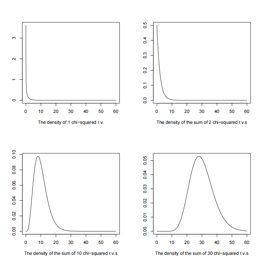
Fig. 14.1 多个卡方分布之和的密度函数

import numpy as np
import matplotlib.pyplot as plt
from scipy import stats


def prompt_distribution() -> str:
    options = {
        "1": "chi2",
        "2": "uniform",
        "3": "exponential",
        "4": "poisson",
    }
    prompt = (
        "请选择基准分布（输入数字）：\n"
        "1. Chi-square distribution (df=2)\n"
        "2. Uniform distribution on [0, 1]\n"
        "3. Exponential distribution (rate=1)\n"
        "4. Poisson distribution (λ=2)\n"
        "你的选择: "
    )
    while True:
        choice = input(prompt).strip()
        if choice in options:
            return options[choice]
        print("请输入 1-4 的数字。")


def read_parameters():
    print("CLT Demo: Comparing sums with different sample sizes")
    dist_key = prompt_distribution()
    return dist_key


def build_pdf(dist_key: str, n: int, x: np.ndarray):
    if dist_key == "chi2":
        return stats.chi2.pdf(x, df=n * 2)
    elif dist_key == "uniform":
        mean = 0.5 * n
        std = np.sqrt(n / 12)
        return stats.norm.pdf(x, loc=mean, scale=max(std, 1e-8))
    elif dist_key == "exponential":
        return stats.gamma.pdf(x, a=n, scale=1)
    else:  # poisson
        mean = 2 * n
        std = np.sqrt(2 * n)
        return stats.norm.pdf(x, loc=mean, scale=max(std, 1e-8))


def determine_range(dist_key: str, n_values):
    if dist_key == "chi2":
        x_min = 0
        x_max = max(12, 4 * max(n_values))
    elif dist_key == "uniform":
        mean = 0.5 * max(n_values)
        std = np.sqrt(max(n_values) / 12)
        x_min = mean - 6 * std
        x_max = mean + 6 * std
    elif dist_key == "exponential":
        x_min = 0
        x_max = max(12, 5 * max(n_values))
    else:  # poisson
        mean = 2 * max(n_values)
        std = np.sqrt(2 * max(n_values))
        x_min = mean - 6 * std
        x_max = mean + 6 * std
    return x_min, x_max


def plot_comparison(dist_key: str):
    n_values = [1, 5, 10, 30]
    x_min, x_max = determine_range(dist_key, n_values)
    x = np.linspace(x_min, x_max, 1200)

    fig, axes = plt.subplots(2, 2, figsize=(10, 7))
    axes = axes.flatten()

    for ax, n in zip(axes, n_values):
        pdf = build_pdf(dist_key, n, x)
        ax.plot(x, pdf, "b-", linewidth=2, label=f"n = {n}")
        ax.set_xlabel("x")
        ax.set_ylabel("Density")
        ax.set_title(f"Sum of {n} variables")
        ax.set_xlim(x_min, x_max)
        ax.set_ylim(bottom=0)
        ax.grid(True, alpha=0.3)
        ax.legend()

    dist_label = {
        "chi2": "chi-square(2)",
        "uniform": "uniform[0,1]",
        "exponential": "exponential(1)",
        "poisson": "poisson(λ=2)",
    }[dist_key]

    fig.suptitle(f"CLT Illustration: summing {dist_label} variables", fontsize=14)
    fig.tight_layout(rect=[0, 0, 1, 0.96])
    plt.show()


def main():
    dist_key = read_parameters()
    plot_comparison(dist_key)


if __name__ == "__main__":
    main()

Remark

随着 \(k\) 的增加， \(S_k\) 的密度函数图像越来越接近正态分布曲线。

对于卡方分布 \(\chi^2(k)\) 而言，其期望和方差分别为

\[ E(S_k)=k, \quad \text{Var}(S_k) = 2k.\]

当 \(k\) 增加时， \(S_k\) 的密度函数的位置右移，且 \(p_{k}(s)\) 的方差也增大。这意味着这个分布的中心趋向 \(\infty\) ，其方差也趋向 \(\infty\) ，分布极不稳定。因此，直接讨论 \(S_k\) 的分布是有困难的。于是，在中心极限定理的研究中均对 \(S_k\) 进行标准化，即

\[ S_k^\ast = \frac{S_k - E(S_k)}{\sqrt{\text{Var}(S_k)}} \]

可以证明

\[\begin{split} \begin{eqnarray*} E(S_k^\ast) = 0\\ \text{Var}(S_k^\ast) = 1 \end{eqnarray*} \end{split}\]

一个很自然的问题是 \(S_k^{\ast}\) 的极限分布是否为标准正态分布 \(N(0,1)\) ?

Question

中心极限定理本身研究的是在什么条件下，随机变量之和的极限分布是正态分布。